Programming a Real Self-Driving Car: Udacity SDC Nanodegree
At the end of my senior year of college while taking a full course load, I also opted to be in the very first group of people taking the Udacity Self-driving Car Nanodegree.
At the time I wrote a post about each of the parts of the nanodegree. I have now combined all of them into one post so it doesn’t take up so much room in the posts section on my website.
Capstone project: Programming a real self-driving car!
Github
Introduction
All of the projects in the Udacity lead up to one final project. In this final project, you team up with up to 4 other people from the program and put your code on Udacity’s real self-driving car.
Parts
Traffic Light Detection
This was the part I worked on. My team split this into two parts
- Transform space. We were supplied the location of the traffic light relative to us. If you know the focal length and a couple other details about the camera, you can figure out which pixels represent the object if you know where in space the object is.
- Classification. We needed to classify the traffic light as red, yellow, or green, so that we would know whether to go or not.
Waypoint Following
The car needs a list of waypoints to follow. In this project, we’re given a list of base way points and the position of the car, and we need to provide a list of waypoints ahead of us so that the car knows what to follow.
Once we know where the traffic lights are and whether they’re red or green, the waypoint updater then cuts off the waypoints at red lights and extends the waypoints to green lights.
Drive-By-Wire
The interface to the car gives goal speed and turning values and the drive-by-wire module is responsible for turning those into throttle and brake. Our team solved this using PID with the steering and throttle individually.
Video
I was lucky enough to be one of the few to see the car run my team’s code in person. Here’s a video of it attempting one loop around.
Semantic Segmentation: Udacity SDC Nanodegree Term 3 Project 2
Github
Introduction
Detecting the boxes surrounding an object is something that works well in certain circumstances, but sometimes you need a higher level of precision. What if you could label each pixel as the type of object it is a part of? That’s where semantic segmentation comes in.
Fully Convolutional Neural Networks
In a normal convolutional neural network, we usually have two parts. The first part is convolutional. This part recognizes shapes. The second part does the dirty work of labeling that shape as one (or one of many) label.
In a fully convolutional network, we don’t have that second part. Instead, after the convolutional part is done, we then reverse the convolutions in order to bring the image back to its original size. This allows us to label each pixel and to keep the information about where in an image each part was.
Path Planning: Udacity SDC Nanodegree Term 3 Project 1
Github
Introduction
In the MPC project we made a car follow a predefined path. In order to do that, though, the car needs a path to follow. In this project we made a smooth path for the car to follow and made it avoid other cars while keeping the correct speed and doing everything smoothly.
The Simulator
This simulator works in a simple way. Every .02 seconds, the car moves to the next dot, so we then know exactly where the car is going to be in the next position.
Logic
- If there is not another car in front of our current car, speed up to the max speed (45mph)
- If there is another car in front of our car, change lanes if possible, and if not, slow down to that car’s speed until there is a lane available or until that car is going faster than our top speed.
Smoothness
- Making a smooth line between waypoints: I used a spline library here. This library creates one smooth path through any points yoyu give it. On each calculation, the car makes a 9-point spline (with the 4 waypoints behind it, the 4 in front of it, and the closest one). It then uses that spline as a reference for where it should be.
- Speeding up smoothly. This is just a matter of slowly increasing velocity. We are increasing velocity at a rate of 2.5m/s^2, or .05m/s per .02s increment.
- Changing lanes smoothly. I decided to do this with a method called the Jerk-Minimizing Trajectory. We take the position we’re at and find the trajectory that gets us from the lane we’re in to the lane we want to be in that reduced jerk the most.
- While turning, there is extra jerk, so when calculating how fast to change lanes we also take into account the jerk from turning within the road.
Feedback from Reviewer
I got some great feedback on this project that I wanted to share here
Greetings Udacian,
Congratulations :star:
I must applaud this great work and I will say I really like the structure of the code and the documentation. This is a clear master-piece and deserves an acknowledgment. Please keep up the great work and remain brilliant.
Video
MPC Controller: Udacity SDC Nanodegree Term 2 Project 5
Github
Introduction
When humans drive, we don’t just look to see how far away from the center of the lane we are and how close to the speed limit we are. We look ahead and slow down if there’s a sharp corner coming up, and we try to do so smoothly. When coming out of a turn, we try to slowly bring the steering wheel to its desired position. And we do so differently depending on if we have a sports car or SUV. Model Predictive Control attempts to replicate this behavior.
The idea is that with a Model Predictive Controller, we look ahead a certain distance and figure out, knowing how quickly we can accelerate and how much we can turn, what the best possible way to get there is. After we have a plan for how to accomplish our goal, we then take the first step, and then recalculate before sending the car another direction.
Model…
A model, in this context, is the computer’s idea of what the car can do. A simple model could assume that the car will never slide and will figure out how much the car will turn when we turn the wheels a certain amount and go a certain distance. A more advanced model will take into account maximum acceleration, maximum grip, and take into account delays.
Predictive…
After we have an idea of what our car will do, we then can take a set of instructions over time and estimate what the car will do if we give it those instructions. The better our model is, the better our prediction is and the better our prediction is, the more accurate our trajectory will be.
Control
Once we have the equation for what the car will do given any set of instructions, we then can use an optimizer tool to figure out the best set of instructions to accomplish our goal. We can also give different weights to multiple goals, such as telling the car to follow a line, but prioritize smoothness over being close to the line, or to prioritize minimal acceleration over being close to the speed limit.
In This Lesson
The model keeps track of 8 variables:
x: the x position of the car, in relation to the map y: the y position of the car, in relation to the map psi: the orientation of the car in relation to the map v: the velocity of the car, in meters/second cte: the cross-track error between the car and the middle of the map epsilon: the difference between the angle of the car and the angle of the track delta: the amount that the car should be turning acceleration: the amount of throttle the car is putting on. These are calculated at each step in .1 second intervals for the next 20 intervals, so the car can plan ahead for the next two seconds. I tried .5 second intervals, but the car just didn’t update fast enough.
In order to figure out where the car has to go, I first convert the global coordinates given by the map into local coordinates to the car. The idea behind this is that the local coordinates are going to have lower numbers and therefore it’s less likely to have inaccuracies due to any conversion imprecision.
The program has a simulated 100ms latency, to account for the fact that in the real world, readings aren’t going to come instantly. In order to combat this, I made it so that the time interval between the dots it predicts is low. The more frequently we’re calculating the things directly ahead of us, the better our accuracy is going to be for the things directly ahead of us.
Video
PID Controller: Udacity SDC Nanodegree Term 2 Part 4
Github
Introduction
PID is one of the most common ways to get an object to get to the place you want it to go. With PID, all you need to do is give the algorithm the error (how far away you are from the goal) and tune 3 parameters to make it smooth. This is easy to implement, moves into position smoothly, and automatically compensates for cases where motor calibration is off (i.e. if you put weight on the end of a motor that’s trying to lift something, the algorithm will naturally give more power to the motor).
PID
In this project, we used PID to make a vehicle turn toward the center line on a track. Here’s how each of the parts of PID relate to a car following a line:
P: Position. This is how far away the car is from the center line. We want to minimize this. I: Integral. This is essentially how much time has been spent on one side of the track (with spending time far away from the track counting more than time close to the center). This will compensate in case the car has a left-turn or right-turn bias. D: Derivative. This is the difference between the angle of the car and the angle of the line. We want the car to be going at the same angle as the line, so we try to minimize the difference. The biggest advantage of PID is that it’s easy to implement and works well in many scenarios. The biggest disadvantage is that it’s reactive (as opposed to proactive), meaning that the car isn’t planning ahead. This makes it hard to make a PID controller that will handle a car going excessive speeds. In my case I couldn’t get the car going consistently over 120mph with a PID controller. For this project, Udacity provided a simulator that would give you the cross-track error (the distance from the center line) and I implemented the PID algorithm to make the car go around the track.
Video
Kidnapped Vehicle (Particle Filter): Udacity SDC Nanodegree Term 2 Project 3
Github
Introduction
Kalman Filters work great, but can be difficult to implement. What if we want an easy way to figure out what the robot is doing without having to figure out a model for it? This is where particle filters come in.
Kidnapped Vehicle
The premise behind this project is that there is a vehicle that has sensors on it, and you need to figure out where it is.
Particle Filter
To figure out where the vehicle is, or ‘localize’ the vehicle, a particle filter follows the following steps:
- Place a bunch of virtual robots around the map in random positions.
- Take measurements with our actual robot.
- Compare the measurements of our actual robot with the measurements that we think each of our virtual robots would have taken
- If this virtual robot’s measurements are similar to what the physical robot’s measurements are, we know that that virtual robot is much more likely to be in the same positon as our physical robot.
- Make a new set of virtual robots, making more robots close to the virtual robots with high probability of being correct.
- Move the physical robot, and simulate movement for each of the virtual robots in the same motion. Then repeat the entire measurement process.
This will eventually give you an estimate for the robot’s location. This can be extended to velocity and acceleration as well.
No Video This Time
Unfortunately because I was in the first cohort, Udacity did not have a visualizer ready for this project.
Unscented Kalman Filter: Udacity SDC Nanodegree Term 2 Project 2
Github
Introduction
Extended Kalman Filters have the problem where they are still linear - the jacobian is essentially a linear approximation. Motion, however, is rarely linear. An Unscented Kalman Filter attempts to fix that.
CTRV Model
In the last project, we assumed the car had a constant velocity. This becomes inaccurate when the car is accelerating or turning. There are a few different models that can take into account acceleration, turning, and other motions. The one we use in this project is the CTRV model which stands for Constant Turn Rate and Velocity. The Unscented Kalman Filter will allow us to account for turning, where this model would screw up the Extended Kalman Filter
Sigma Points
The reason we can only use linear functions in an Extended Kalman Filter is that it depends on keeping a gaussian disctibution for how sure it is of the points. When we apply the transformations that an Extended Kalman Filter uses, it turns that function into a non-gaussian distribution, which means that we may have two or more ideas of where the true value is.
Instead of applying our non-linear function directly, what an Unscented Kalman Filter does is is finds points that are representative of each of the variables we’re changing and the gaussian function representing them. It then transforms those points, and from that transformation we can now create a new gaussian distribution. It’s difficult to explain without a full lesson (you can find full lessons on Youtube if you’re interested), but the basic idea is that this new gaussian is representative of your confidence in the new, non-linear function. This tends to work better than an Extended Kalman Filter in places where motion changes a lot.
Video
If you compare this one to the video in the previous lesson, you’ll notice that the green triangles are much closer to the circle and less spread out than in the last lesson.
Extended Kalman Filter: Udacity SDC Nanodegree Term 2 Project 1
Github
Introduction
From sensors, you tend to get a lot of noisy data. When a sensor tells you that you’re in one place one second and in another place another second, you have to decide which ones is right. This is where a Kalman filter comes in.
Kalman Filters
A Kalman Filter keeps track of confidence levels in measurements. Usually you have two parts: A model of what should be happening, and the data from the sensor on what the measurements actually are.
Take, for example, the situation where the sensor is getting data every second. At the first second, it says an object is 2 meters away, and at the second second, it says the object is 3 meters away. Your model might predict that the object will be 4 meters away at the third second. What happens, then when the third second comes and the sensor says the object is 4.1 meters away? Do you trust the sensor, knowing that the sensor could be slightly off, or do you trust your model, knowing that your model could be slightly off? A Kalman filter will figure out which one to trust more and give a value that’s usually somewhere between the sensor value and your predicted value.
Extended Kalman Filter
The normal Kalman filter has a problem where it predicts things linearly. This means that, for example, at time t0 an object is 1 meter away, at t1 the object is 4 meters away, and t2 the object is 9 meters away, that it will have a hard time predicting that the next object will be 16 meters away. Extended Kalman Filters were created to help alleviate that. With an extended kalman filter, you can use a nonlinear function to model the behavior you expect.
Unfortunately, thanks to the way Kalman filters use variances, it’s not as easy as sticking the function in and being done with it. You have to use the jacobian matrix for the function, which is a matrix with every possible partial derivative. This will approximate the function as a linear function and is often a good enough approximation to keep estimate good.
Sensor Fusion
The two parts of a Kalman filter, the data and the model, can be extended with multiple sensors. The model will stay the same, but we can update the data from multiple sensors together.
For this project, we emulated the data from a lidar and a radar. There are some key differenced between the two. A lidar will only directly give you position. If you want to figure out how fast an object is going, you have to take two measurements at two different times and figure out the difference between those two measurements, then divide that by the time between the two measurements. A radar, on the other hand, can directly measure speed. This means that when you’re updating the data with the radar, you can give speed directly instead of looking at your model to determine speed. A radar has the drawback of being noisier than a lidar, so the data is going to be less consistent. If we use these two together, we can get a better idea of what the truth is. The filter will now figure out how confident it is in the model, the lidar, and the radar individually, and output one value that’s a compromise between the three.
Video
Here’s a video of the kalman filter working. The red dots are lidar measurements, blue are radar measurements, and green is where the EKF thinks we are.
Vehicle Detection: Udacity SDC Nanodegree Term 1 Project 5
Github
Introduction
Figuring out where cars are in a picture is less easy than it sounds. First, you need a classifier that can correctly figure out what is and is not a car. Second, you have to figure out where those cars are in a way that is both accurate and computationally inexpensive. This is what we learned in the fifth project of the SDC Nanodegree.
Pipeline
This particular project did not have a lot of leeway for how to complete it. Here is the pipeline Udacity suggested that I also used:
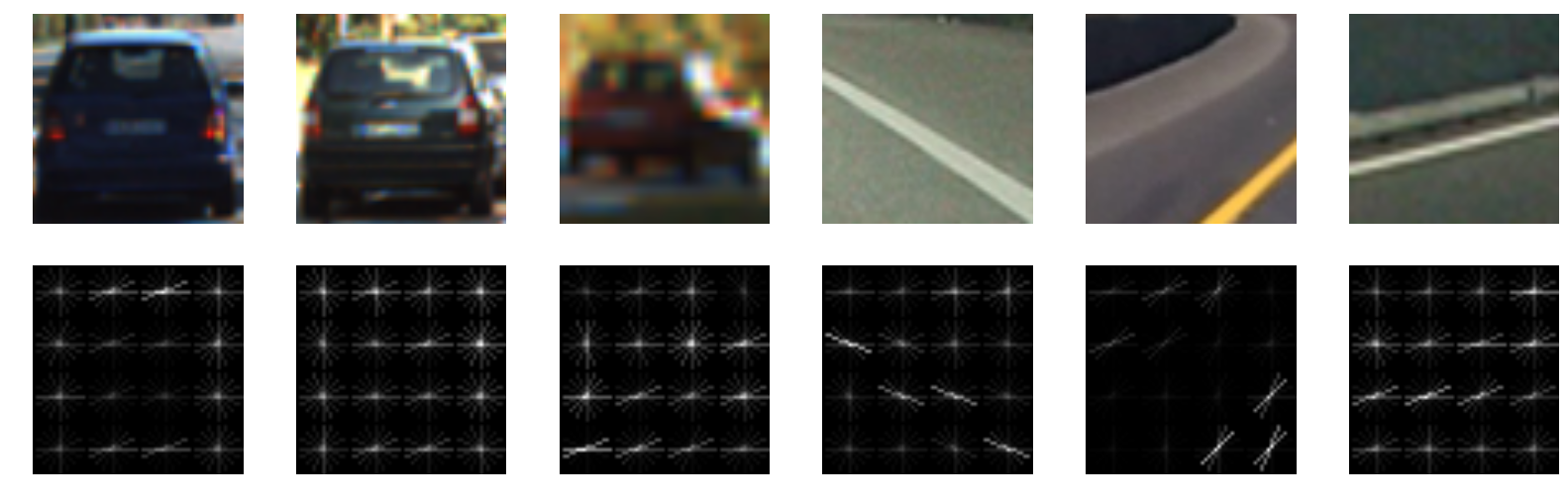
Histogram of Oriented Gradients
This is an algorithm that will figure out how the color is changing in each part of an image and by how much is that color changing. In the pictures below, the gradients and their magnitudes are represented by white lines in a black box. The algorithm separates the picture into smaller boxes and figures out the gradient for each box. You’ll notice that the lanes are represented well by gradients of approximately the same angle as the lane.
Support Vector Machine
An SVM is a machine learning algorithm that takes in a list of features and classifies them. In this case, each of the features was the output of the histogram of oriented gradients. An SVM can be used in many of the same ways as a neural network, without having to worry about layer sizes. It can be customized with different kernels to fit more complex data. It can also be much quicker to train than a neural network.
In my training set, I used around 60,000 images of cars and not cars.
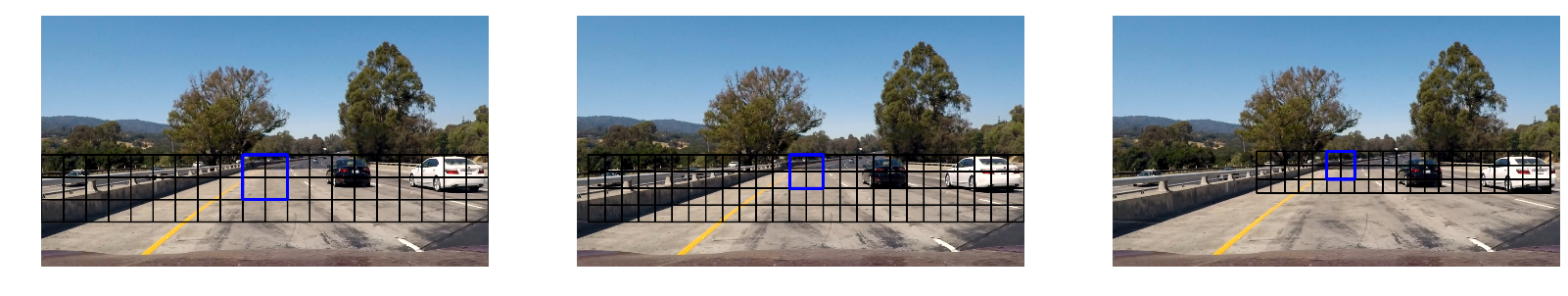
Sliding Window
After we have an SVM that will classify a car consistently, we can use a sliding window method to figure out where in the image the car is.
The idea is simple: We have a classifier that can figure out whether an image is a car or not. We then take that classifier and run it on various parts of the image. Because the car could be at any distance, we also take different sized samples and run the classifier on them.
Hotboxes
After we’ve run the sliding window algorithm, we now have a bunch of boxes that probably have a car in them. We now need to take those boxes and figure out which ones are accurate. We can do that by finding the areas where lots of boxes intersect. We call this method ‘hotboxes’.
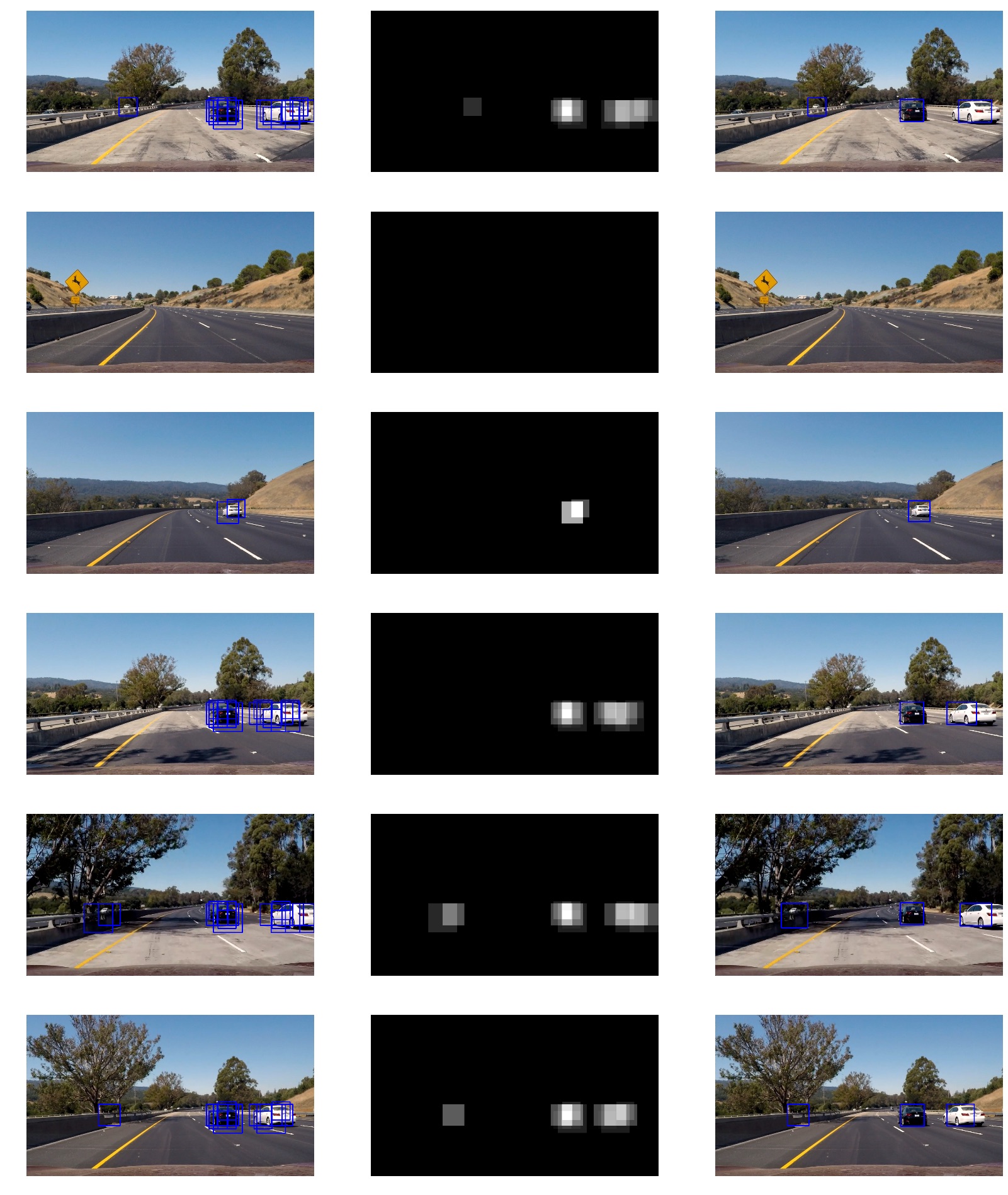
Video
Advanced Lane Lines: Udacity SDC Nanodegree Term 1 Project 4
Github
Introduction
In project 1 of term 1, we made a pipeline that can detect lane lines, but only straight lane lines. In a real car, you need something more complicated to figure out exactly where the lane lines are. This project is an extension of the first project in term 1. In this project, we use perspective transforms and thresholding to fit lines to the lanes we see.
The Pipeline
Here I will go through each of the methods we learned in this lesson and give an example of how we get from start to finish
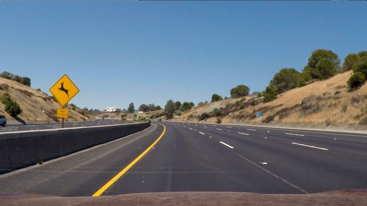
We will start with our original image:
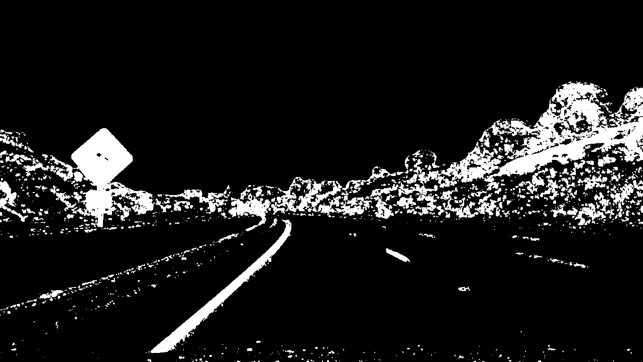
Color thresholding
We know that our lane lines will be one of two colors: yellow or white. We can use that knowledge to signal out only the yellow or white parts of the image. We say that if this part of the image is above a certain percentage of yellow, we make it white, and if it’s below that, we make it black.
Sobel Operator
Once we have the white and yellow parts of the image, can use the Sobel Operator to find edges. The sobel operator looks at a bunch of pixels and finds the gradient between them. In other words, it highlights the place where the color change, and highlights big changes in color more than smaller places. We know that the color is going to change a lot in out lane lines, so this will help them stand out.
After color thresholding and sobel operator, this is what the image looks like:
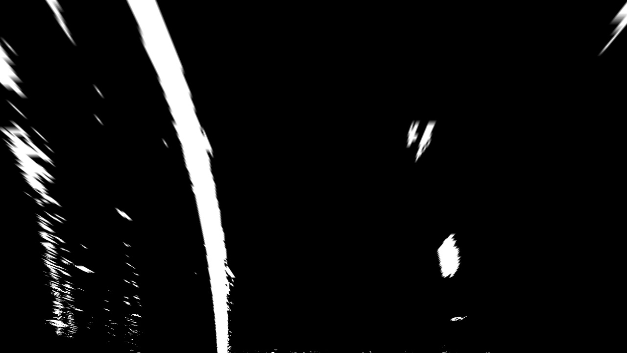
Perspective Transform
In order to find curves to fit these lane lines, we want to be looking at them from above. There is a tool available with OpenCV to transform an image so that it looks like you’re looking from another direction. Here’s what the image looks like after a persepective transform:
From here, we try to fit two curves to the pixels in the right palce. This is the hard part. I made my pipeline look at the left and right sides of the pictures and find places with a lot of vertical pixels. I then used a sliding window to find the pixels above that, then adusted the sliding window to halfway between the mean of the new pixels and the mean of the old pixels.
Once we figure out which pixels to use for our lines, it’s easy to fit a polynomial curve to them and then highlight the area between the two curves. Here’s what it looks like after this process:

After we’ve done that, we undo the perspective transform that we did earlier so that the picture is in the same perspective as earlier.
If I then put the old picture back in, here’s what it looks like
Now I do that for every frame of the video. Here’s what it looks like:
Behavioral Cloning: Udacity SDC Nanodegree Term 1 Project 3
Github
Introduction
Behavioral cloning is a machine learning technique used to train an agent (whether that’s simulated or a robot) to act by looking at what a human has told the robot to do in similar situations. In this project, we drove a car around a virtual environment, collected data on how I drove, then used a neural network to make the car drive the same way.
Process
My initial model took in two laps’ worth of data around the track in the simulator. With this model, the car would turn left when it needed to turn left and turn right when it needed to turn right, but it would turn at such extreme angles that it couldn’t go very fast.
I found two things that helped this: increasing the learning rate, which smoothed out the actions, and changing the optimizer to an Adam optimizer instead of a regular Gradient Descent optimizer.
With these two changes, the car was much smoother, but would not turn sharp enough. It looked as if the car had overfit for straightaways.
I did two things to counteract this. First, I took away 50% of the data where the steering angle was less than 10 degrees. Second, I recorded myself taking some more sharp turns.
Now, instead of retraining the model with the above data, I took the existing model, and extended the training with the new data. The idea behind this was that I liked how smooth the existing model was, I just wanted to make small adjustments to it. It worked well, and after this the car would go full speed around the track. I didn’t think that was good enough, though.
The car still seemed to try and go left on the straightways and then correct itself to go right occasionally. This caused me to think that it was overfit going to the left. I flipped all of the training data and added it to the original training data, and then continued training the model on the new doubled data. After 8 epochs, the model now went straight on straightways.
Conclusion
I ended up very happy with a model that could go around the track at the highest speed the simulator would allow it, since this very much surpassed the requirements for the project. I learned a lot, like when to continue training an already trained network and when to start from scratch, how important training data is, and how hyperparameters affect your neural network.
Video
First attempt
Final attempt
Traffic Sign Classifier: Udacity SDC Nanodegree Term 1 Project 2
Github
Introduction
This project was an introduction to CNNs in tensorflow. Udacity gives the student some suggestions on what a convolutional neural network looks like and then the student goes and implements that on their own
My solution
Here’s what my final CNN looked like. It was trained on the dataset provied my Udacity
Input: 32x32x3 (a 32x32 pixel color image) Layer1: 2D convolution with an output of 28x28x6, and a pooling layer of kernel size 2x2 with a stride of 2 for an output of 14x14x6 Layer2: 2D convolution with output size 10x10x16, and a pooling layer with kernel size 2x2 for an output of 5x5x16 Fully Connected 0: Flatten layer 2 Fully connected 1: Matrix multiply with input 400 and output 120, then a relu activation Fully connected 2: Matrix multiply with input 120 and output 84, then a relu activation Output layer: Matrix Multiply with input 84 and output 43 (for 43 possible labels)
This was trained on the dataset provided by Udacity (https://d17h27t6h515a5.cloudfront.net/topher/2017/February/5898cd6f_traffic-signs-data/traffic-signs-data.zip) for an accuracy of 94.2% of the validation set
Finding Lane Lines: Udacity SDC Nanodegree Term 1 Project 1
Github
Background
I was picked when I was a senior in college to be one of the first 500 people in the first cohort of Udacity’s Self-Driving Car Nanodegree. I was told later that I was picked because I had taken many online classes before and that not many people applied to take the nanodegree while simultaneously taking college courses.
Introduction
This project is an introduction to OpenCV. The goal is to find lane lines on a video feed of a car driving on a highway
Finding Lane Lines
CV Algorithms
In order to finish this project, we were taught some classical computer vision techniques, such as:
Canny Edge Detection
This algorithm finds where edges in the picture might be, and brings them back as a list of lines. Parameters one might adjust include how long the minimum and maximum lines must be and how sensitive the algorithm is to deciding whether something is a line or not.
Hough transform
Hough Transform is another name for taking lines in x,y coordinate space and turning them into r, theta coordinate space. From here, we can easily find lines that are close to each other and going the same direction, so that if we have many similar lines from the output of the canny edge detection, we can combine those into one line
Pipeline
From picture to video, here’s what my final pipeline looks like:
- Greyscale the image
- Gaussian blur the greyscaled image, with kernel size 5
- Apply canny edge detection with a low threshold of 0 and a high threshold of 200
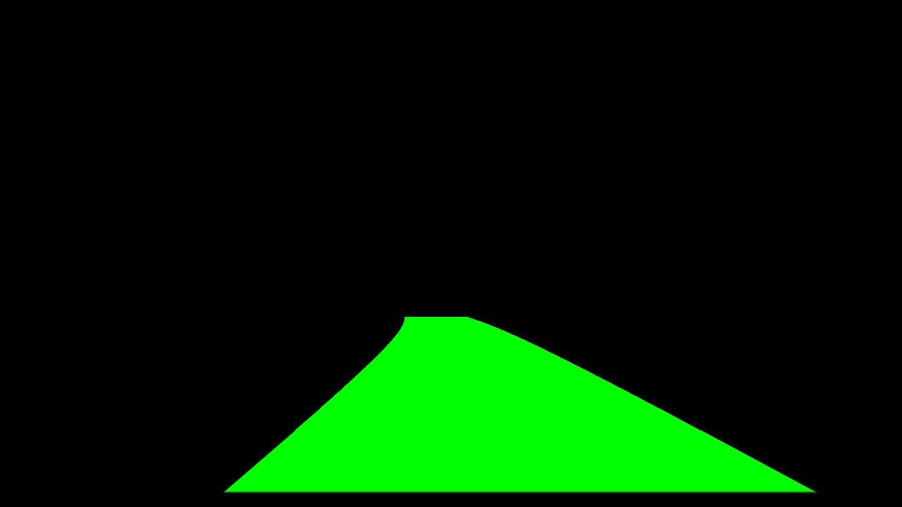
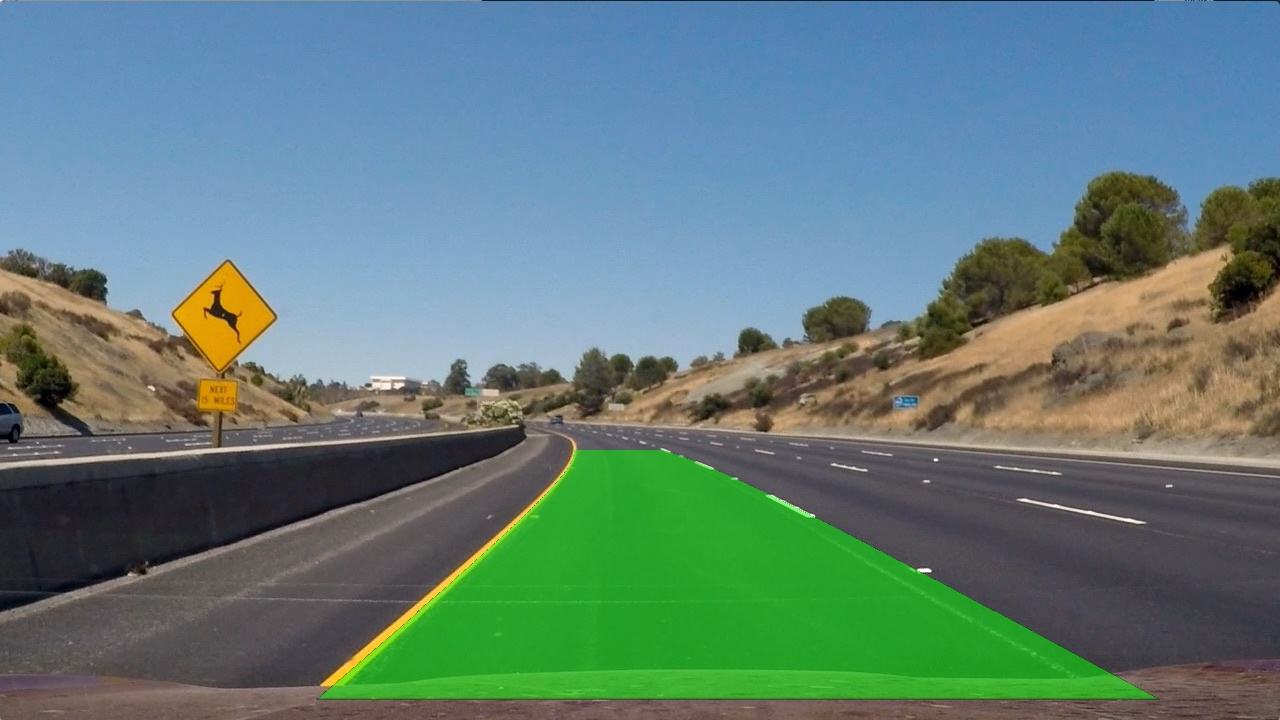
- Apply a mask to the places where we expect the road might be.
- Use hough transform to find lines, with a minimum line length of 100 pixels and maximum gap between lines being 100 pixels as well.
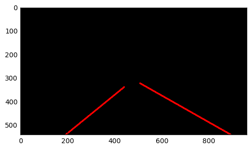
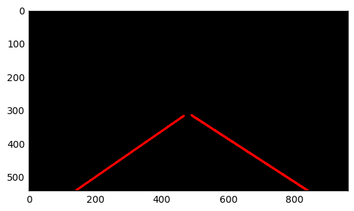
- Split the lines into two groups: the lines with positive slope (left lines) and the lines with negative slope (right lines)
- Find the standard deviation of each set and filter out any lines not within one standard deviation
- Find the mean line of all remaining lines. This is our new line.